Sutton and Barto: Problem 13.1

tl;dr

• This post solves a problem from Reinforcement Learning: An Introduction by Richard S. Sutton and Andrew G. Barto.
• The problem asked for an exact symbolic expression for the optimal probability of selecting the right action in a gridworld scenario.
• The approach to solve this problem involves use of Markov chains.
• The solution to this equation in the interval [0,1] is $p=2-\sqrt{2}\approx 0.59$, which matches the book’s solution.

In this page I solve a problem from the book Reinforcement Learning: An Introduction by Richard S. Sutton and Andrew G. Barto. It’s really a good book, although the writing style is a bit dry for my taste. I was reading the chapter 13 on Policy Gradient Methods since I want to understand the theory behind Actor-Critic algorithms.

I share this problem for two reasons: I spent quite some time solving it and I want to test the math rendering capabilities of the Jekyll theme I am using for this blog. Furthermore, it might be useful for someone else trying to solve the same problem.

To understand the problem, first I’ll introduce some context. Most algorithms that are used to learn a policy $\pi(s)$ to achieve some task (e.g winning a game) are based on the idea of estimating the value function $v(a | s)$ and then taking the action that maximizes this value:

\[\pi(s) = \arg\max_a v(a | s)\]

This is the idea behind Q-learning, SARSA, etc. Then, to ensure exploration, a random-greedy policy is used, in which with probability $\epsilon$ a random action is taken instead of the greedy one. However, in some cases this method will not converge to the optimal policy. For example, in a game like paper-rock-scissors in which the optimal policy is to choose randomly so your opponent cannot predict your next move, the greedy policy will always choose the action with the highest value (i.e. the action that has happened to win more often in the past). A smart enough opponent may discover this and exploit it to always choose the action that beats the greedy policy whenever there is a value difference between the actions. This book illustrates this issue with a better example in which an agent is trying to reach a goal in a grid world. In the book they explain it better than I could possibly do, so I’ll just put the excerpt:

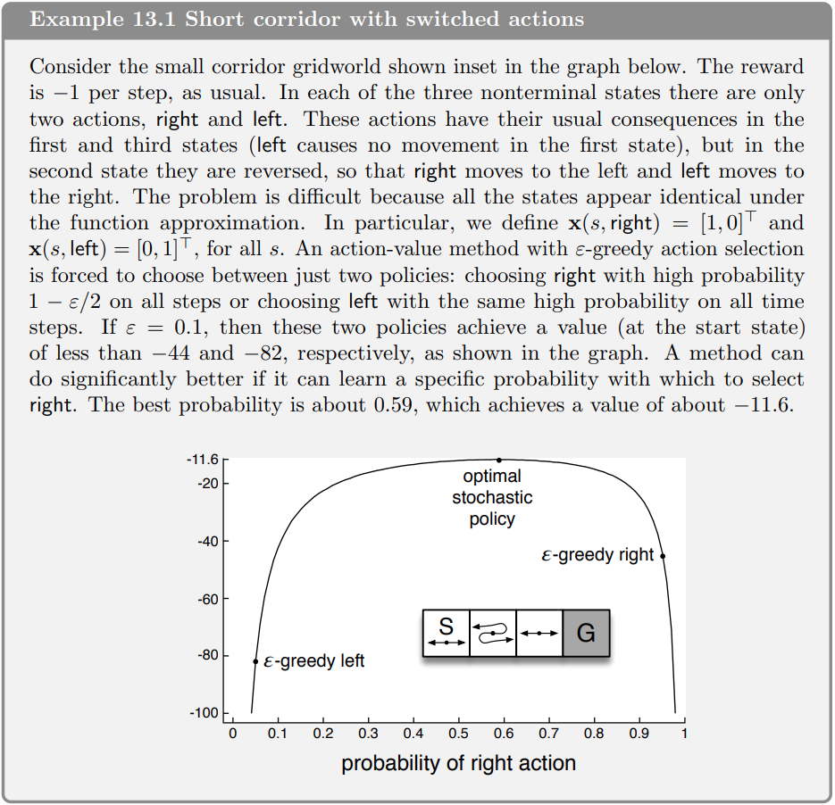
Then the exercise is the following:

Exercise 13.1 Use your knowledge of the gridworld and its dynamics to determine an exact symbolic expression for the optimal probability of selecting the right action in Example 13.1.

I haven’t read most of the chapters on this book yet, so I am not sure if there is some section that explains how to tackle gridworld problems, although I am quite sure they are used extensively in the book to illustrate other examples. Nonetheless, I wanted to solve this problem by myself to prove that I still keep some basic skills in math. I’ve always been terrible at solving probability and statistical problems, so it was quite a challenge for me. But I managed to solve it and I had some fun in the process. I’ll illustrate my solution and my reasoning process now.

I never had a course on probability or stochastic processes, so my set of tools to solve this problem is quite limited. However, I do know what a Markov chain is and this process, since the agent does not have any memory or knowledge about the state of the world, can be modeled as one. So to get a better visualization of the process I drew the following Markov chain representing the process:

The goal to solve this problem is to express as a function of the probability $p$ of the agent taking the action right the expected number of steps for the agent to reach the terminal state 4 from the initial state 1. At first glance, I don’t see any obvious way of calculating the expected number of steps from two distant states in a Markov chain. However, it seems relatively easy to calculate the expected number of steps from the initial state 1 to the state 2. If we think about it, it’s like a biased flip coin in which the coin lands heads with probability $p$ and tails with probability $1-p$. The expected number of steps for this transition $E_{1\rightarrow 2}$ is just the expected number of tries until the coin lands heads. Then to calculate $E_{1\rightarrow 2}$ we just need to calculate the average of the lengths of each possible sequence of flips that ends in heads weighted by the probability of each sequence.

Let’s go back to the gridworld and introduce a new notation that will be useful for the next steps. Let’s denote by $\mathcal{S}^{1 \rightarrow 2}$ the set of all sequences actions that by starting in state 1 end in state 2 and never go through state 2 twice. For example, the sequence $s_1 = \lbrace\rightarrow\rbrace$ belongs to $\mathcal{S}^{1 \rightarrow 2}$. Another sequence that belongs to this set is $s_2 = \lbrace\leftarrow, \rightarrow\rbrace$. In fact, any sequence of $\mathcal{S}^{1\rightarrow 2}$ consists of a number $n-1$ of actions $\leftarrow$ followed by a final action $\rightarrow$. If we denote by $|s|$ the length of a sequence $s$, then the expected number of steps for the transition is: \(E_{1\rightarrow 2} = \sum_{s \in \mathcal{S}^{1 \rightarrow 2}} p_s |s|\) where $p_s$ is the probability of the sequence $s$. It’s more, this equation is true for any transition between two states of a markov chain. We can just swap the indices of the states and the equation will still be valid: \(E_{i\rightarrow j} = \sum_{s \in \mathcal{S}^{i \rightarrow j}} p_s |s|\) The problem now is to find $p_s$ and $|s|$ for each sequence $s$ and perform the sum.

In the case of $E_{1\rightarrow 2}$ this is easy:

\[E_{1\rightarrow 2} =\sum_{n = 1}^{\infty} \underbrace{(1-p)^{n-1} p}_{p_s} \underbrace{n}_{|s|} = \sum_{m=0}^{\infty} (1-p)^m p(m+1) = p \left( \sum_{m=0}^{\infty} (1-p)^m m + \sum_{m=0}^{\infty} (1-p)^m \right)\]

Now we have to calculate those two series. The second one is just the geometric series, this is:

\[\sum_{m=0}^{\infty} (1-p)^m = \frac{1}{1-(1-p)} = \frac{1}{p}\]

The second one is a bit more complicated. We can use the formula for the geometric series and the linearity of the derivative operator:

\[\sum_{m=0}^{\infty} (1-p)^{m} m = (1-p)\sum_{m=0}^{\infty} (1-p)^{m-1} m = -(1-p)\frac{d}{dp} \sum_{m=0}^{\infty} (1-p)^{m} = \frac{1-p}{p^2}\]

Then:

\[E_{1\rightarrow 2} = p \left( \frac{1-p}{p^2} + \frac{1}{p} \right) = \frac{1}{p}\]

Which is the correct answer for the expected number of trials until a biased coin lands heads. Now we would like to use the same reasoning to calculate $E_{1\rightarrow 4}$. However, I could not find a way to express the sum $\sum_{s\in \mathcal{S}^{1 \rightarrow 4}} p_s |s|$ analytically. However, we can use the fact that:

\[E_{1\rightarrow 4} = E_{1\rightarrow 2} + E_{2\rightarrow 3} + E_{3\rightarrow 4}\]

and hope that $E_{2\rightarrow 3}$ and $E_{3\rightarrow4}$ are easy to calculate. Let’s start with $E_{2\rightarrow 3}$.

This case is similar to $E_{1\rightarrow 2}$, but now we have to take into account the fact that the agent can go back to state 1. Each time the agent goes back to state 1, this will, on average, add a number of steps $E_{1\rightarrow2}$ to the count. Let’s try to count the first sequences of $\mathcal{S}^{2\rightarrow3}$. The first sequence $s_1 = \lbrace\leftarrow\rbrace$ has $|s_1|=1$ and probability $p_{s_1}=1-p$.

The second sequence

\[s_2 = \lbrace \rightarrow, \bar{s}_{1\rightarrow2}, \leftarrow \rbrace\]

has an expected number of steps equal to

\[<|s_2|>=E_{1 \rightarrow 2} + 2\]

and probability

\[p_{s_2}=p(1-p)\]

Note that I introduced the notation $\bar{s}_{i\rightarrow j}$ to denote a randomly sampled sequence from the set $\mathcal{S}^{i\rightarrow j}$

The third sequence

\[s_3 = \lbrace\rightarrow, \bar{s}_{1\rightarrow2}, \rightarrow, \bar{s}_{1\rightarrow 2}, \leftarrow \rbrace\]

has an expected number of steps equal to

\[<|s_3|> = 3 + 2E_{1\rightarrow2}\]

and probability

\[p_{s_3}=p^2(1-p)\]

In general, it is easy to see that \(<|s_n|>=n + (n-1)E_{1\rightarrow 2}\) and \(p_{s_n}=p^{n-1}(1-p)\)

Then, we can obtain $E_{2\rightarrow3}$ by calculating the series:

\[\begin{aligned} E_{2\rightarrow3} &= \sum_{n=1}^{\infty} p_{s_n} \\ &= \sum_{n=1}^{\infty} p^{n-1}(1-p) (n + (n-1)E_{1\rightarrow 2}) \\ &= \sum_{n=1}^{\infty} p^{n-1}(1-p)(n + (n-1)\frac{1}{p}) \\ &= \sum_{m=0}^{\infty} p^m (1-p)(m+1+\frac{m}{p}) \\ &= (1-p)\left(\sum_{m=0}^{\infty} mp^m + \sum_{m=0}^{\infty} p^m + \frac{1}{p}\sum_{m=0}^{\infty} mp^m \right) \\ &= (1-p)\left( \frac{p}{(1-p)^2} + \frac{1}{1-p} + \frac{p}{p(1-p)^2} \right) =\frac{2}{1-p} \end{aligned}\]

To calculate $E_{3\rightarrow 4}$ the set up is identical. We just need to change $p \leftarrow (1-p)$ and $E_{1\rightarrow 2} \leftarrow E_{2\rightarrow 3}$. If we do so we find that:

\[E_{3\rightarrow 4} = \frac{3}{p}\]

Now to calculate $E_{1\rightarrow 4}$ we just need to add the three expected number of steps:

\[E_{1\rightarrow 4} = E_{1\rightarrow 2} + E_{2\rightarrow 3} + E_{3\rightarrow 4} = \frac{1}{p} + \frac{2}{1-p} + \frac{3}{p} = \frac{4}{p} + \frac{2}{1-p}\]

To find the optimal value of $p$ we just need to find the value of $p$ that minimizes $E_{1\rightarrow 4}$. To do it we calculate the derivative:

\[\frac{d}{dp} E_{1\rightarrow 4} = -\frac{4}{p^2} + \frac{2}{(1-p)^2}\]

If we set it to zero we obtain the equation:

\[p^2 -4p + 2 = 0\]

The solution of this equation tha lies in the interval $[0,1]$ is $p=2-\sqrt{2}\approx 0.59$, which is the same value that the book provides.