How Progress is Made - Part 2

This article is long ( ~ 1h read), so I have split it into three parts of ~ 20 minutes each.

• Part 1: Introduction, Definition of Progress, Episodic vs Continuous Tasks
• Part 2: Progress by search, structure of search spaces, why induction works
• Part 3: The role of predictive models, infrastructure and competition (coming soon)

Progress by search, structure of search spaces, why induction works

Progress by search

Now that we have a clear understanding of the different types of tasks, we can discuss the search methods that lead to progress. A particularly interesting read on this topic is The Bitter Lesson. In this article, Rich Sutton argues that the most important lesson that can be drawn from the history of AI is that general methods that leverage computation are ultimately the most effective. I mostly agree with this statement, but I think it’s important to not lose sight of the fact that information is more general than it seems and systems can extrapolate from different data sources by using inductive reasoning.

In this section, I’ll talk about some search methods. It won’t be extensive, but it will be useful to convey the general principles and limitations of search. There are countless books written about optimization, so I won’t go into the details of each method.

Exhaustive search

This is the most straightforward search method. It consists of testing every single strategy in the strategy space $S$ and selecting the one that performs best.

Obviously, this method is only feasible for small strategy spaces. For example, in a small town with few roads, we can test every possible route to find the shortest one. However, as the number of roads increases, the number of possible routes explodes superpolynomially, and the exhaustive search becomes infeasible (this is known as the traveling salesman problem).

Random search

Random search involves randomly selecting candidate solutions from the strategy space $S$ and evaluating their performance. It does not rely on any information about previously evaluated solutions.

While this method may seem naive, sometimes it is at good as it gets. It’s in fact optimal for problems in which the search space has no structure. But, what does it mean for a search space to have structure? This is a term that you often hear in the context of optimization, but I’ve never seen it formally defined. I’m sure there are hundreds of formal papers about this topic, but I’m a physicist and I don’t know them. So, I’ll try to define it here. What I’ll present is not a formal definition, it will be sloppy math at best, but I think it will be “nice” to provide some intuition about the concept. If you know a formal definition of structure of search spaces, please let me know in the comments.

Structure of search spaces

We say that the strategy space $ S $ possesses a “structure” with respect to $ M_T $ if there exists a statistical dependency among the performances $ M_T(s_i) $ for the different $ s_i \in S $. I like to think about this in the terms of mutual information. Let $ X $ and $ Y $ be random variables representing $ M_T(s_i) $ and $ M_T(s_j) $ for $ s_i, s_j \in S $ and $ i \neq j $. Then $ S $ is said to lack structure if and only if

\[I(X; Y) = 0, \quad \forall s_i, s_j \in S, i \neq j,\]

where $ I $ is the mutual information between two random variables.

Mutual information is a measure of the mutual dependence between two random variables. It quantifies the amount of information (bits) obtained about one random variable after observing the other random variable.

In cases where there’s no structure it’s straightforward to see why random search can be an effective method, since any systematic approach that tries to infer the performance of one strategy based on another will be futile. Instead, uniformly sampling strategies from the search space is as good as any other method.

Grid example

Let me illustrate the idea with the following optimization problem. We have a grid of 20x20 pixels, with values ranging from 0 to 255, 0 being black and 255 being white. We are interested in the coordinates of the brightest pixel. To get the brightness of a pixel, we can call a oracle function $M(x, y)$ that returns the brightness of the pixel at coordinates $(x, y)$. So in this case, our strategy space is $S = \{(x, y) \in \mathbb{N}^2 | 0 \leq x, y \leq 19\}$, and our performance metric is the brightness $M(x, y)$.

Now imagine we have 3 different grids.

• Grid 1: Single white pixel All pixels are black except for one, which is white.

• Grid 2: Uniformly distributed pixels The brightness of each pixel is randomly sampled from a uniform distribution between 0 and 255.

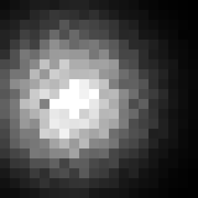
• Grid 3: Normally distributed pixels The brightness of each pixel is randomly sampled from a Gaussian distribution with the origin at a random point in the grid.

From these grids, can you tell which one has no structure? How would you find the brightest pixel knowing that you can only call the function $M(x, y)$ to get the brightness of a pixel one at a time? Please take a moment to think about it before continuing the article, since it’s a good exercise to understand the concept of structure in search spaces.

Grid 1: Single white pixel

This grid possesses structure. In this case, there exists a unique $ (x_{\text{max}}, y_{\text{max}}) $ such that $ M(x_{\text{max}}, y_{\text{max}}) = 255 $, while $ M(x, y) = 0 $ for all other $ (x, y) $. Here, $ I(X; Y) \neq 0 $ because knowing $ M(x, y) $ for one $ (x, y) $ gives full information about $ M(x’, y’) $ for all $ x’ \neq x $ and $ y’ \neq y $.

Nonetheless, note that structure may not offer any advantage, since in this case no strategy can improve the time complexity of exhaustive search.

Interesting fact: Grover’s algorithm is a quantum algorithm that can find the brightest pixel in a grid of size $N$ in $\mathcal{O}(N)$ steps, assuming we can evaluate the performance metric $M(x, y)$ with a quantum oracle (which is rarely possible). This is a quadratic speedup over the $\mathcal{O}(N^2)$ steps required by exhaustive search.

Grid 2: Uniformly distributed pixels

This grid has no structure. The value of each pixel is independently and uniformly sampled from the range $[0, 255]$. Let $X$ and $Y$ be defined as before, by definition of the grid $P(X,Y) = P(X)P(Y)$, and therefore $I(X; Y) = 0$.

If the search space has no structure, then random or exhaustive search are as good as we can get. It doesn’t matter what method we use: as long as we don’t repeat strategies, all strategies are equally likely to find the brightest pixel in a given number of trials.

Grid 3: Normally distributed pixels

In Grid 3, pixel brightness follows a Gaussian distribution centered at a specific point $(x_{\text{center}}, y_{\text{center}}) $ and governed by $b(x, y) \sim \mathcal{N}(\mu, \sigma^2) $, where $\mu(x, y) = A \exp\left(-\frac{(x-x_{\text{center}})^2 + (y-y_{\text{center}})^2}{2\sigma^2}\right) $. The mutual information $I(X; Y) $ between any two pixel brightness values $M(x_1, y_1) $ and $M(x_2, y_2) $ is non-zero for nearby pixels due to this Gaussian structure. Thus, the search space possesses structure, enabling optimization techniques like hill-climbing to efficiently locate the maximal brightness.

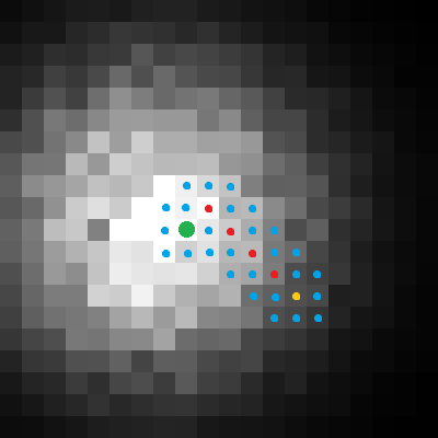
In the following figure you can see the path taken by a high-climbing method to find the brightest pixel in Grid 3. The yellow dot is the starting point, the red dots are the nodes the algorithm picked for checking the value of the pixels around, the blue dots are the explored pixels, and the green dot is the brightest pixel found.

Structured Nature of Complex Search Spaces

Consider the Traveling Salesman Problem (TSP), which involves finding the shortest route through $N$ cities. While the optimal path might be complex to describe—I think $\sim \log{n!}$ in terms of Kolmogorov complexity—the search space is not uniformly random. Instead, there’s a form of ‘useful redundancy’ (i.e. mutual information). For instance, if two cities are geographically close, any optimal or near-optimal solution is likely to visit them consecutively. You can quantify this by observing the distribution of total distances when you swap two adjacent cities in an otherwise fixed route. Typically, such a change results in a small variation in total distance, indicating that ‘nearby’ solutions in the search space also yield ‘nearby’ outcomes.

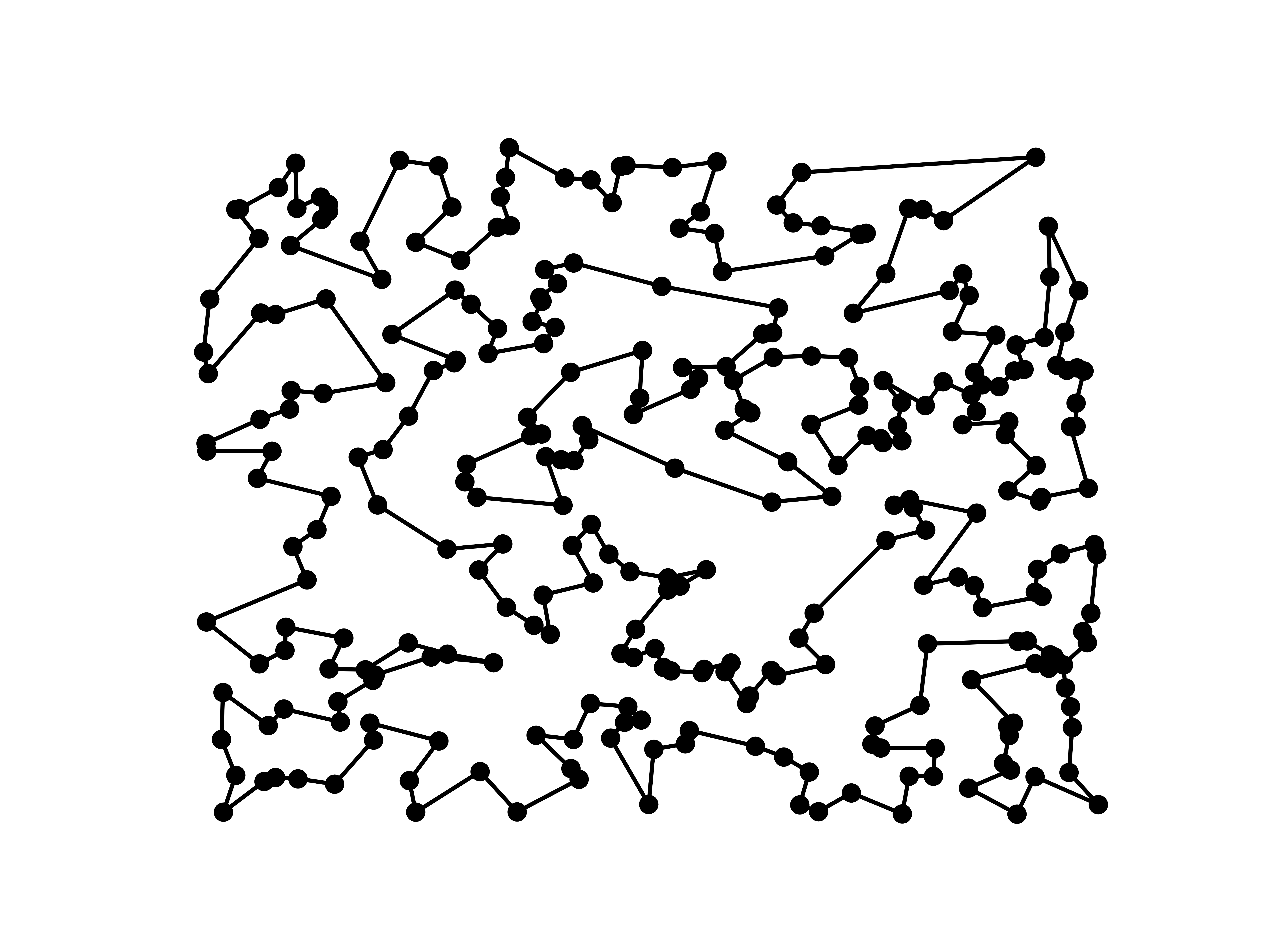
Let’s explore this in more detail with a concrete example. Below you can observe the solution provided by a simple monotonic hill-climbing algorithm for the TSP of 300 randomly located cities. The algorithm starts with a random route and then iteratively swaps two adjacent cities and keeps the swap that results in the shortest route. The algorithm stops when it can’t find a better route after a certain number of iterations.

The Hamming distance between two strings of equal length is the number of positions at which the corresponding symbols are different. In other words, it measures the minimum number of substitutions required to change one string into the other. In this case, we can express the route as a sequence of cities, where each city is represented by a number. For example, the route $[1, 2, 3, 4]$ means that the first city visited is city 1, the second city visited is city 2, and so on. The Hamming distance between two routes is the number of cities that are in different positions in the two routes. For example, the Hamming distance between $[1, 2, 3, 4]$ and $[1, 3, 2, 4]$ is 2, since the cities 2 and 3 are in different positions in the two routes.

Now, we can explicitly observe the structure of the solution space. First we need a way to quantify the similarity between two solutions. A straightforward choice here is to use the Hamming distance between two sequences. Next, we sample random permutations of the optimal route and group them by their Hamming distance to our optimal solution. We then plot the average length of the routes for each group. The results are illustrated in the figure below:.

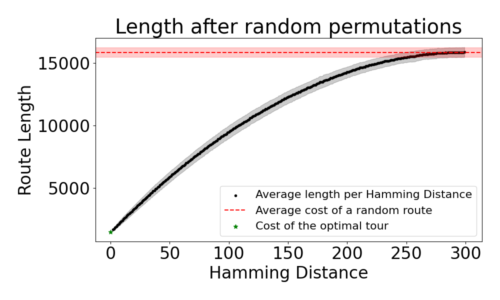
Interestingly, the graph shows that as the Hamming distance to the optimal solution increases, the average route length also increases until it matches the average length of a completely random route.

Let’s see a different example. Take an aircraft: it can be understood as the solution of a problem that involves optimizing the distribution of atoms in space to achieve a desired functionality (flying). Swapping or slightly altering the position of atoms in non-critical components of a plane, like a seat cover, will hardly impact the aircraft’s overall performance. In terms of search space, this means that there’s a cluster of similar, nearly-as-good solutions surrounding any optimal configuration. Humans take advantage of this structure by using modular designs that allow for an abstract compressed description of the aircraft. You don’t need to specify the exact position of every atom in the seat cover, you just need to specify the type of material and the general shape. And this is possible because the structure of the search space allows for it. If this were not the case and you would need to specify the exact position of every atom.

In both these concrete cases, a key principle stands out: small alterations to complex strategies often yield similarly effective results. This isn’t accidental. When a problem demands a high degree of complexity for its solution, the configuration space often manifests clusters of high-performing solutions that are closely related, thereby exhibiting high mutual information between them. This is often needed to ensure robustness and fault tolerance that allows the strategies to perform correctly when slight alterations occur. For example, if the layout of atoms in an aircraft were extremely sensitive to small perturbations, then the aircraft would be very fragile and prone to failure.

The innate structure of complex search spaces isn’t just a mathematical curiosity; it’s a key property that enables both natural and human-engineered systems to operate effectively and adaptively.

Exploiting Structure: Why Induction Works?

Imagine you are a toddler that never has seen an electrical stove. You touch the stove at one point and you burn. Wow. However, you are a curious kid and you touch again the stove in a different point. Burned again. You are starting to learn something. While you may not fully understand the underlying reasons, you’re intuitively picking up on a pattern: touching the stove leads to pain. This is the essence of induction: drawing general conclusions from specific observations.

The essence of inductive reasoning is about learning from these specific experiences and updating our beliefs accordingly. In this case, the toddler starts with a belief (based on prior experiences) that touching new things is generally safe. However, after being burned twice by the stove, they update this belief. They start to generalize that touching the stove leads to pain.

This learning process is a fundamental aspect of how our brains work, and it has evolutionary advantages. For our ancestors, quickly learning from specific instances (like the rustling of bushes often preceding a predator’s attack) was crucial for survival.

An interesting question then arises: Could it be that only certain spots on the stove are hot? While it’s theoretically possible, it’s improbable. Given the vast number of points on the stove’s surface, the chances of accidentally touching the only hot spots are slim. Therefore, it’s more reasonable to infer that a significant part of the stove, if not all of it, is likely to cause burns. This rationale is a simplistic illustration of Solomonoff’s theory of inductive inference. It prioritizes simpler explanations over more complex ones, implying a correlation between the complexity of a hypothesis and the Bayesian probability of it being true.

Ok, but what does this have to do with exploiting structure in search spaces? The key idea is that when a search space possesses structure, observations from one section of the space can offer insights about other sections. This is because we operate under the Bayesian assumption that it’s more probable for the structure to be consistently spread across the entire space than for it to be confined only to the portion we’ve observed.

Exploiting Structure: Local search

When we talk about exploiting structure, one of the primary methods that comes to mind is local search. This method operates on the assumption that nearby solutions in the search space are likely to have similar performances. And this is generally true, as we saw in the previous examples. In the case of the TSP, swapping two adjacent cities in a route is likely to result in a similar total distance. In the case of the aircraft, swapping two adjacent atoms in the seat cover is unlikely to affect the aircraft’s overall performance. In other words, if you find a good solution, then slightly altering it will probably lead to another good (or possibly better) solution.

Local search works by starting with an initial solution and then iteratively making small changes to it. At each step, the algorithm evaluates these changes and decides whether to accept or reject them based on whether they improve the solution or not. The classic example of a local search algorithm is the hill-climbing algorithm, which always moves towards the direction of increasing performance, much like climbing towards the peak of a hill.

However, this is not effective in spaces where the good solutions are isolated or where there are many local maxima or minima. In such cases, the algorithm can easily get stuck in a local optimum and fail to find the best overall solution.

Depending on the use of information, we can classify local search algorithms into three categories:

Zeroth order methods

Zeroth order methods in optimization refer to techniques that do not require the computation of derivatives. These methods only rely on the evaluation of the function being optimized. Examples include the aforementioned random search and exhaustive search, as well as more sophisticated techniques like genetic algorithms and simulated annealing.

These methods are particularly useful when the function is complex, non-differentiable, or when its derivatives are too costly to compute. They are also robust to the peculiarities of the search space, such as non-convexity or the presence of many local optima.

First order methods

First order methods use the first derivative (gradient) of the function to guide the search. The most common example of a first order method is gradient descent, where you iteratively move in the direction opposite to the gradient of the function at the current point.

These methods are more efficient than zeroth order methods because they use additional information about the structure of the search space. However, they require the performance function to be differentiable, and their performance can be significantly affected by factors like the choice of the step size and the initial starting point.

n-th order methods

N-th order methods use higher-order derivatives to guide the search. These methods can be more efficient than first order methods because they can take into account the curvature of the function, not just its slope.

However, computing higher-order derivatives is often computationally expensive and can be numerically unstable.

Problems of local search, global search and the importance of communication

One of the main challenges with local search methods is the presence of local optima. These are points in the search space where a solution is better than neighboring solutions, but not necessarily the best overall solution. When an algorithm reaches a local optimum, it can get “trapped” and fail to explore other parts of the search space that might contain a better solution.

This issue is particularly acute in complex search spaces with many peaks and valleys. In such spaces, the likelihood of encountering local optima is high, and the algorithm needs a strategy to escape these traps. Researchers often introduce additional mechanisms to help the algorithm escape local optima. For example, in gradient descent, the step size can be adjusted to allow the algorithm to jump over valleys and reach higher peaks. Another common approach is to introduce random perturbations to the algorithm’s behavior to help it explore the search space more broadly.

To overcome this issue, we can use global search methods. These methods involve running multiple local search algorithms in parallel, each starting from a different initial point. The idea is that by exploring the search space from different starting points, we can increase the chances of finding a better overall solution.

In Naruto Shippuden, at some point in the story, Naruto needs to learn a new jutsu called the Rasenshuriken but he is pressed by time and needs to learn it as quickly as possible. So, he uses a technique called Kage Bunshin no Jutsu to create multiple copies of himself and learn the jutsu in parallel. The idea works because the clones have a shared memory after they are dispelled, so the experience of each clone is shared with the others. Naruto is essentially using a form of global search to learn the jutsu. Different clones explore different ways of using chakra to create the Rasenshuriken, and the knowledge acquired by each clone is shared with the others. This allows Naruto to learn the jutsu much faster than he would have been able to do alone.

In the context of complex tasks with general agents, global search methods translate to collaboration and communication. Each agent can be seen as a local search algorithm that explores a specific part of the search space. By sharing information about their experiences, agents can help each other escape local optima and find better solutions.

In speedrunning, the fact that every player have to share a video of their run, forces the competitors to share information about their strategies, which constitutes a effective form of global search.

Search Superspace and General Search Models

Humans are very general problem solvers. How can we achieve this? The answer lies partly in our capacity to abstract patterns from specific instances and apply them universally based again on Solomonoff’s theory of inductive inference. Patterns that emerge from specific problem domains are projected by our minds as likely characteristics of related problems, even those we have yet to observe. It’s this inductive reasoning that allows humans not only to cope with a particular local search space but to make educated guesses and predictions across varied domains of problems.

In the context of search spaces, this means that humans and, by extension, human-designed algorithms and agents, can employ the knowledge gained from one search environment to inform strategies in another. While a local search environment may be highly specialized, the inductive generalizations drawn from it are not necessarily confined to that space alone. They can be leveraged across different search spaces, shaping a form of ‘search superspace’—a higher-dimensional space encompassing the commonalities among the various problems.

This leads to the concept of a General Search Model: a model that is not bound by the specificities of a problem’s search space and instead operates on the premise of generalized patterns and principles learned from multiple search domains. It recognizes the structured nature of complex search spaces and the mutual information that exists between high-performing solutions.

In essence, just as humans have developed the skill to recognize the stove as uniformly hot and thus generalize this to all direct contact with it, a General Search Model can recognize the commonalities between different search spaces and apply the same principles to all of them. These generalizations are likely to work due to the Solomonoff’s theory of inductive inference.